Figures 13.6 and 13.7

[ASKurz]

In Section 13.3.2, Average behavior of sequential tests, Kruschke presented simulations of outcomes based on various stopping rules (p-values, Bayes factors, and so on). From the text, we read:

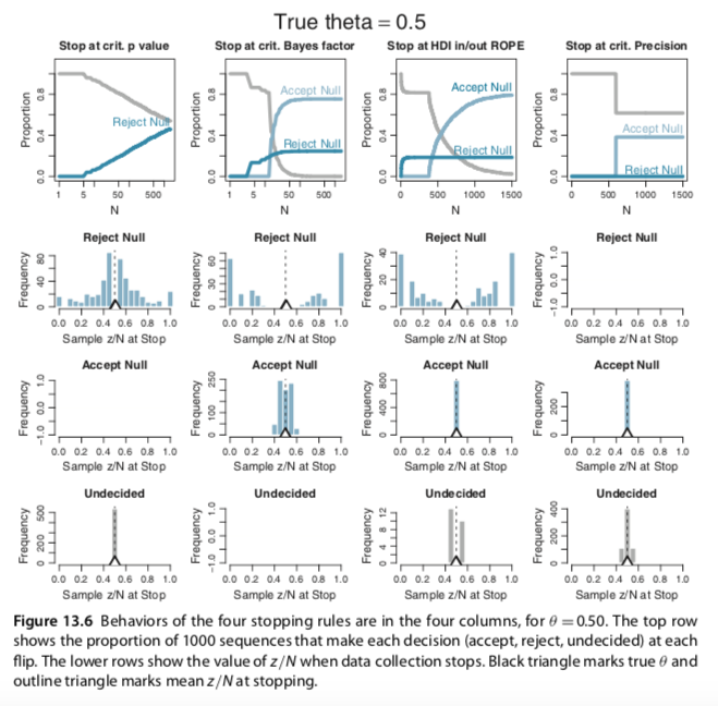
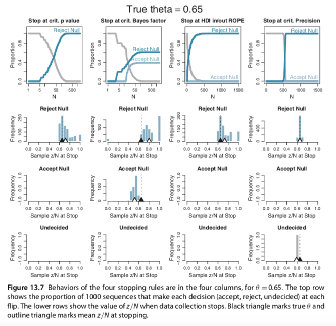
The plots in Figures 13.6 and 13.7 were produced by running 1000 random sequences like those shown in Figures 13.4 and 13.5. For each of the 1000 sequences, the simulation kept track of where in the sequence each stopping rule would stop, what decision it would make at that point, and the value of z/N at that point. Each sequence was allowed to continue up to 1500 flips. Figure 13.6 is for when the null hypothesis is true, with θ = 0.50. Figure 13.7 is for when the null hypothesis is false with θ = 0.65. Within each figure, the upper row plots the proportion of the 1000 sequences that have come to each decision by the Nth flip. One curve plots the proportion of sequences that have stopped and decided to accept the null, another curve plots the proportion of sequences that have stopped and decided to reject the null, and a third curve plots the remaining proportion of undecided sequences. The lower rows plot histograms of the 1000 values of z/N at stopping. The true value of θ is plotted as a black triangle, and the mean of the z/N values is plotted as an outline triangle.

Consider Figure 13.6 for which the null hypothesis is true, with θ = 0.50. The top left plot shows decisions by the p value. You can see that as N increases, more and more of the sequences have falsely rejected the null. The abscissa shows N on a logarithmic scale, so you see that the proportion of sequences that falsely rejects the null rises linearly on log(N). If the sequences had been allowed to extend beyond 1500 flips, the proportion of false rejections would continue to rise. This phenomenon has been called “sampling to reach a foregone conclusion” (Anscombe, 1954).

The second panel of the top row (Figure 13.6) shows the decisions reached by the Bayes’ factor (BF). Unlike the p value, the BF reaches an asymptotic false alarm rate far less than 100%; in this case the asymptote is just over 20%. The BF correctly accepts the null, eventually, for the remaining sequences. The abscissa is displayed on a logarithmic scale because most of the decisions are made fairly early in the sequence.

The third panel of the top row (Figure 13.6) shows the decisions reached by the HDI- with-ROPE criterion. Like the BF, the HDI-with-ROPE rule reaches an asymptotic false alarm rate far below 100%, in this case just under 20%. The HDI-with-ROPE rule eventually accepts the null in all the remaining sequences, although it can take a large N to reach the required precision. As has been emphasized in Figure 12.4, p. 347, the HDI-with-ROPE criterion only accepts the null value when there is high precision in the estimate, whereas the BF can accept the null hypothesis even when there is little precision in the parameter estimate. (And, of course, the BF by itself does not provide an estimate of the parameter.)

The fourth panel of the top row (Figure 13.6) shows the decisions reached by stopping at a criterial precision. Nearly all sequences reach the criterial decision at about the same N. At that point, about 40% of the sequences have an HDI that falls within the ROPE, whence the null value is accepted. None of the HDIs falls outside the ROPE because the estimate has almost certainly converged to a value near the correct null value when the precision is high. In other words, there is a 0% false alarm rate.

The lower rows (Figure 13.6) show the value of z/N when the sequence is stopped. In the left column, you can see that for stopping at p < 0.05 when the null is rejected, the sample z/N can only be significantly above or below the true value of θ = 0.5. For stopping at the limiting N of 1500, before encountering p < 0.05 and remaining undecided, the sample z/N tends to be very close to the true value of θ = 0.5.

The second column (Figure 13.6), for the BF, shows that the sample z/N is quite far from θ = 0.5 when the null hypothesis is rejected. Importantly, the sample z/N can also be noticeably off of θ = 0.5 when the null hypothesis is accepted. The third column, for the HDI-with-ROPE, shows similar outcomes when rejecting the null value, but gives very accurate estimates when accepting the null value. This makes sense, of course, because the HDI-with-ROPE rule only accepts the null value when it is precisely estimated within the ROPE. The fourth column, for stopping at criterial precision, of course shows accurate estimates. (pp. 399--391).

He then went on to explain Figure 13.7. For the sake of space, I'll omit that prose. Here is Kruschke's Figure 13.6:

And here is Kruschke's Figure 13.7:

At present, I’m not sure how to pull off the simulations necessary to generate the figures. If you have the chops, please share. If at all possible tidyverse-oriented workflows are preferred.