Conditional Probability

Introduction

In the previous lessons and labs, you learned about some fundamentals of probability theory, along with basic combinatorics such as permutations and combinations. You'll now extend your knowledge of probability by learning about Conditional Probability. You'll see how Conditional Probability is extremely important in Statistics, and the foundation of many applications. Understanding conditional probability is essential when exploring fields in Machine Learning and Artificial Intelligence.

In this lesson, you'll learn about conditional probability, what it is, and how and when to use it. Later on, you'll see how this simple idea becomes a key component in most statistical machine learning algorithms.

Objectives

You will be able to:

• Differentiate between independent and dependent events
• Use the multiplication rule to find the probability of the intersection of two events
• Use conditional probability to explain the Product Rule, Chain Rule, and Bayes Theorem

Events and Sample Space

Before introducing you to specific event types, let's do a quick recap of the notion of event and sample space.

An event is the outcome of an experiment, for example, obtaining heads when tossing of a coin or getting 3 after a dice roll. Note: an event can also be a collection of different events grouped together (or a so-called compound event), e.g. getting a 3 twice when rolling a dice twice.

A sample space is a collection of every single possible outcome in a trial, generally represented by $\Omega$. The sample space for 1 random dice throw is {1,2,3,4,5,6}.

As you remember for the previous lessons, we can combine events and sample space to compute event probability.

You'll learn about 3 important event types: independent, disjoint, and dependent events.

Independent Events

Events $A$ and $B$ are independent when the occurrence of $A$ has no effect on whether $B$ will occur (or not).

Consider the following independent events:

• Getting heads after flipping a coin and getting a 5 after throwing a fair dice
• Choosing a marble from a container and getting heads after flipping a coin

Two independent events

Formally, events A and B are independent if:

• $P(A \cap B) = P(A)P(B)$

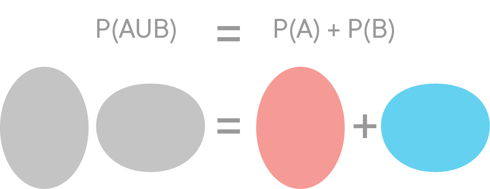
The probability of A or B occurring, $P (A \cup B)$, is given by the addition rule of probability:

$$P (A \cup B) = P(A) + P(B) - P(A \cap B).$$

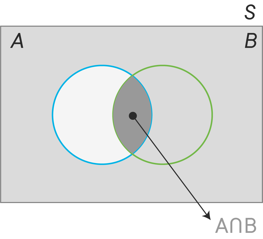
We subtract the intersection of the two events to avoid over-counting. See the diagram below for some intuition:

Thus, in the case of two independent events, by substitution,

$$P (A \cup B) = P(A) + P(B) - P(A)P(B)$$

Thus, in the case of two independent events, by substitution,

$$P (A \cup B) = P(A) + P(B) - P(A)P(B).$$

Three independent events

Three events, A, B and C, are independent if:

• $P(A \cap B) = P(A)P(B)$
• $P(A \cap C) = P(A)P(C)$
• $P(B \cap C) = P(B)P(C)$
• $P(A \cap B \cap C) = P(A)P(B)P(C)$

So you need both pairwise independence and three-way independence

Disjoint Events

Events $A$ and $B$ are disjoint if $A$ occurring means that $B$ cannot occur.

Disjoint events are mutually exclusive. $P (A \cap B)$ is empty.

Dependent Events

Events $A$ and $B$ are dependent when the occurrence of $A$ somehow has an effect on whether $B$ will occur (or not).

Now things start getting a bit more interesting.

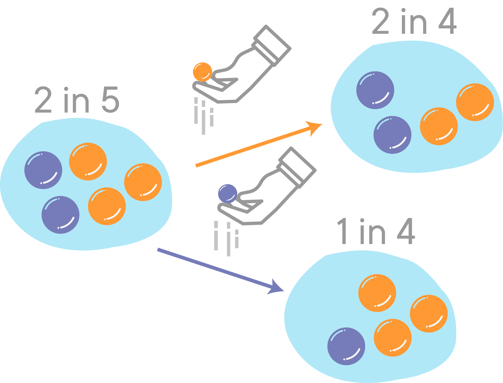
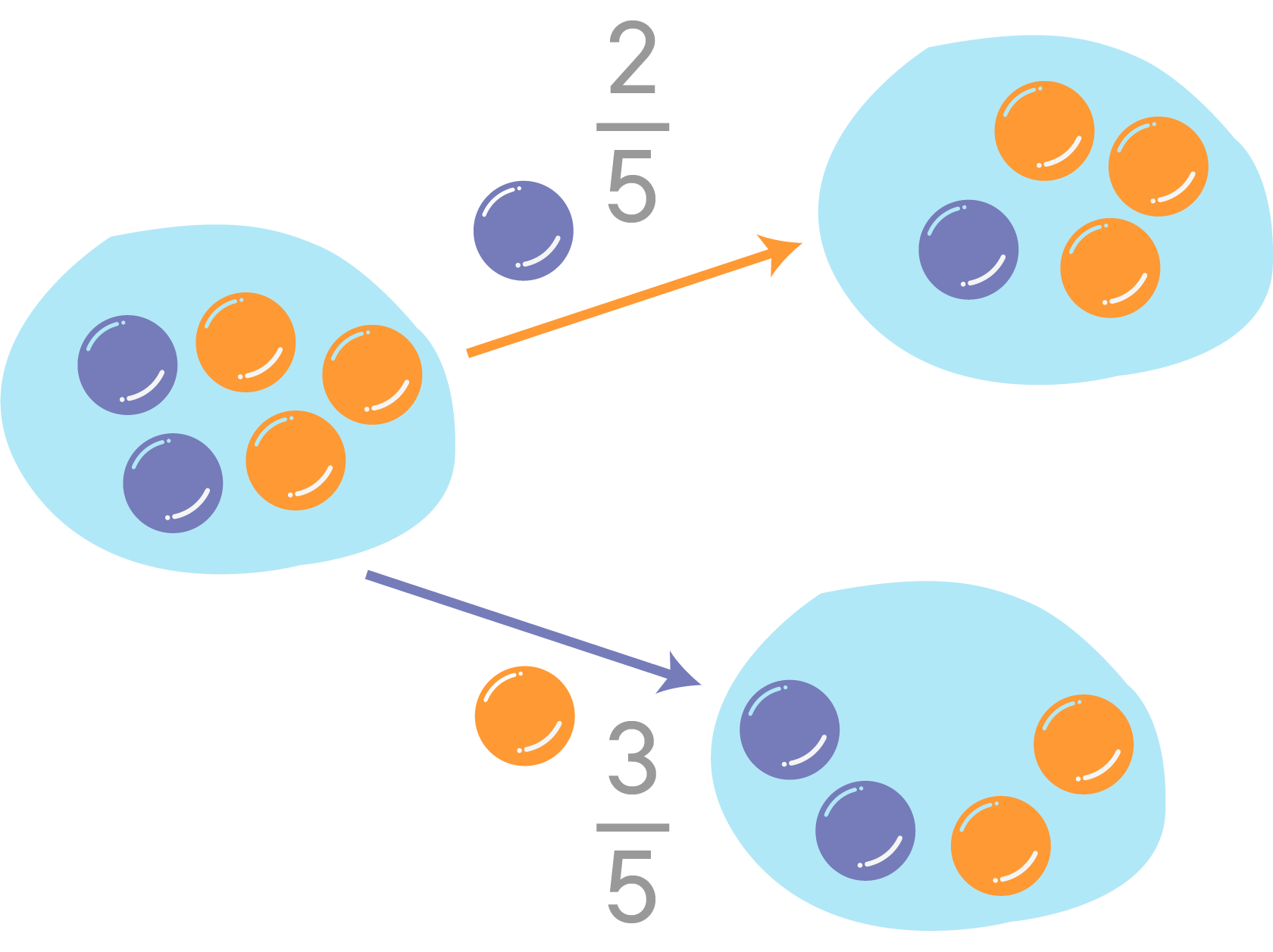
Let's look at an example. Let's say event $A$ is taking an orange or purple marble out of a jar. The jar contains 3 orange and 2 purple marbles.

The probability of getting a purple marble is $\dfrac{2}{5}$ and getting an orange marble is $\dfrac{3}{5}$.

At that point, one marble is taken out and we now take another marble from the jar (event $B$).

Here you can see that our second event is dependent on the outcome of the first draw.

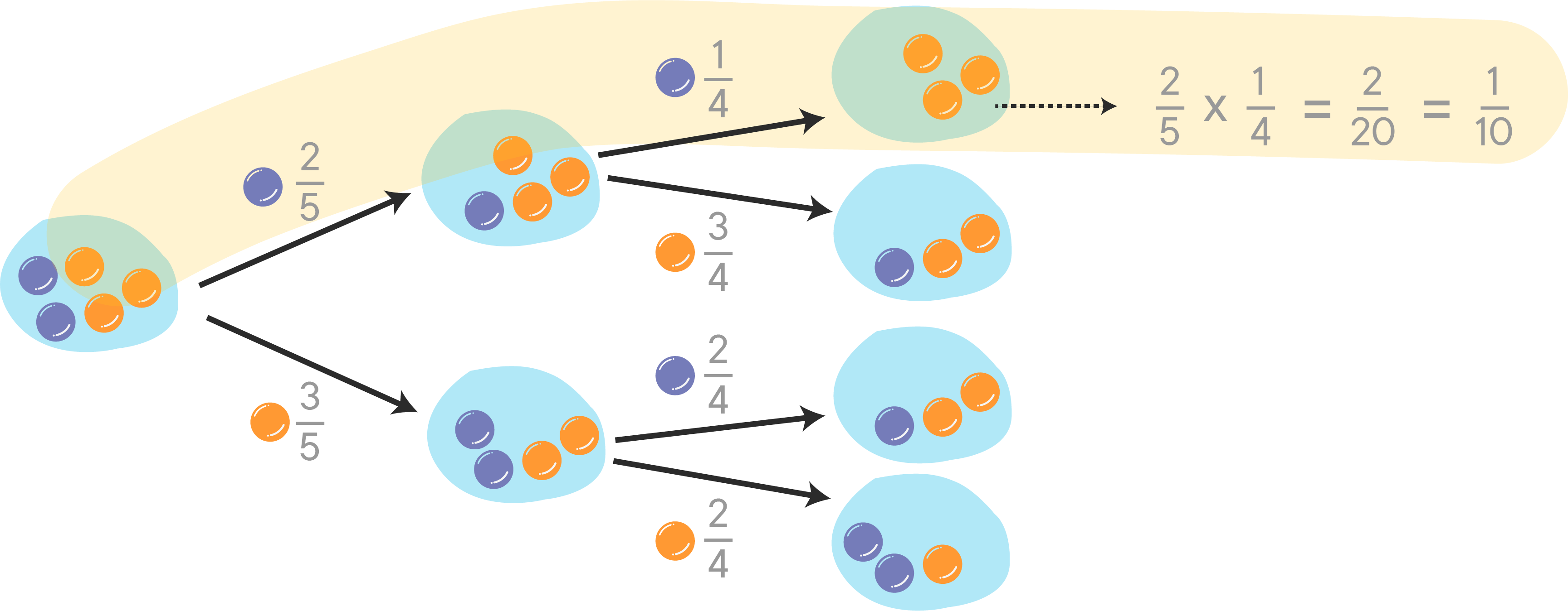
• If we drew an orange marble first, the probability of getting a purple marble for event B is $\dfrac{2}{4}$.
• If we saw a purple marble first, however, the probability of seeing a purple in the second trial is $\dfrac{1}{4}$.

In simple terms, the probability of seeing an event $B$ in the second trial depends on the outcome $A$ of the first trial. We say that $P(B)$ is conditional on $P(A)$.

A tree diagram can be used to explore all possible events.

Conditional Probability

Conditional probability emerges when the outcome a trial may influence the results of the upcoming trials.

While calculating the probability of the second event (event $B$) given that the primary event (event $A$) has just happened, we say that the probability of event $B$ relies on the occurrence of event $A$.

Here are some more examples:

• Drawing a 2nd Ace from a deck of cards given that the first card you drew was an Ace.
• Finding the probability of liking "The Matrix" given that you know this person likes science fiction.

Let's say that $P(A)$ is the event we are interested in, and this event depends on a certain event $B$ that has happened.

The conditional probability (Probability of $A$ given $B$) can be written as: $$ P (A \mid B) = \dfrac{P(A \cap B)}{P(B)}$$

$P(A|B)$, is the probability A given that $B$ has just happened.

Understanding this formula may be easier if you look at two simple Venn Diagrams and use the multiplication rule. Here's how to derive this formula:

Step 1: Write out the multiplication rule:

• $P(A \cap B)= P(B)*P(A\mid B)$

Step 2: Divide both sides of the equation by P(B):

• $\dfrac{P(A \cap B)}{ P(B)} = \dfrac{P(B)*P(A\mid B)}{P(B)}$

Step 3: Cancel P(B) on the right side of the equation:

• $\dfrac{P(A \cap B)}{P(B)} = P(A \mid B)$

Step 4: This is of course equal to:

• $ P(A \mid B)=\dfrac{P(A \cap B)}{P(B)} $

And this is our conditional probability formula.

There are a few variations and theorems that are related to and/or results of this conditional probability formula. The most important ones are: the product rule, the chain rule and Bayes Theorem

Theorem 1 - Product Rule

The product rule was used to derive the conditional probability formula above, but is often used in situations where the conditional probability is easy to compute, but the probability of intersections of events isn't.

The intersection of events $A$ and $B$ can be given by:

\begin{align} P(A \cap B) = P(B) P(A \mid B) = P(A) P(B \mid A) \end{align}

Remember that if $A$ and $B$ are independent, then conditioning on $B$ means nothing (and vice-versa) so $P(A|B) = P(A)$, and $P(A \cap B) = P(A) P(B)$.

Theorem 2 - Chain Rule

The chain rule (also called the general product rule) permits the calculation of any member of the joint distribution of a set of random variables using only conditional probabilities.

Recall the product rule:

$P(A \cap B) = P(A \mid B) P(B)$

When you extend this for three variables:

$P(A\cap B \cap C) = P(A\cap( B \cap C)) = P(A\mid B \cap C) P(B \cap C) = P(A \mid B \cap C) P(B \mid C) P(C)$

And you can keep extending this to $n$ variables:

$$P(A_1 \cap A_2 \cap \ldots \cap A_n) = P(A_1 \mid A_2 \cap \ldots\cap A_n) P(A_2 \mid A_3 \cap \ldots \cap \ A_n) P(A_{n-1}|A_n) P(A_n)$$

This idea is known as the chain rule.

If on the other hand you have disjoint events $C_1, C_2,...,C_m$ such that $C_1\cup C_2\cup ··· \cup C_m = \Omega$, the probability of any event can be decomposed as:

\begin{align} P(A) = P(A \mid C_1)P(C_1) + P(A \mid C_2)P(C_2) + \ldots + P(A \mid C_m)P(C_m) \end{align}

Theorem 3 - Bayes Theorem

The Bayes theorem, which is the outcome of this section. Below is the formula that we will dig deeper into in upcoming lessons.

\begin{align} P(A|B) = \frac{P(B|A)P(A)}{P(B)} \text{- this follows from Theorem 1} \end{align}

Additional note: the complement of an event

You learned about (absolute and relative) complements before, but the complement of an event is also applicable to conditional probabilities.

The basic rule is:

$P(A) + P(A') = 1$

with A' being the complement of A.

Similarly, extending this to conditional probabilities:

$P(A|B) + P(A'|B) = 1$

Example : An Aspiring Data Scientist's Dilemma

Let's see a very simple use of the conditional probability formula. A data scientist comes across the following infographic:

Curious as data scientists are, he starts collecting data about weather conditions and his own mood.

Consider the data in the following table, recorded over a month with 50 days by our data scientist. On each day he recorded whether it was sunny or Cloudy, and whether his mood was good or not.

	Sunny weather	Cloudy weather
Good mood	14	11
Bad mood	2	23

He wants to now know if his mood had anything to do with the weather on a particular day and how he can calculate the probability of having a good mood given the weather conditions.

If he picked a day at random from the 50 days on record, what is the probability that he was in a good mood on that day, $P(G)$?

• The sample space is 50 days here
• The event space is "good mood", so $14 + 11 = 25$.
• $P(G) = \dfrac{25}{50} = 0.5$

What is the probability that the day chosen was a Sunny day, $P(S)$?

• The sample space is still 50 days
• It was sunny on $14 + 2 = 16$
• $P(S) = \dfrac{16}{50} = 0.32$

What is the probability of having a good mood given it's a sunny day $P(G \mid S)$ ?

• $P(G \mid S) = \dfrac{P(G \cap S)}{ P(S)}$, so we need to calculate $P(G \cap S)$ first.

• $P(G \cap S)$ consists of sunny days in which he is in a good mood. There were 14 of them, so $P(G \cap S) = \dfrac{14}{50}$

• Therefore $P(G \mid S) =\dfrac{\frac{14}{50}}{\frac{16}{50}} = 0.875 $

The infographic had some truth in it indeed. There's a $87.5%$ chance that our curious data scientist would be in good mood on a sunny day.

The data scientist is satisfied and thinks the outcome is comforting.

Surfing the Internet, however, he comes across a Garth Stein quote. Although not very scientific, this raises his curiosity further. The quote goes as follows:

$\large \text{"That which is around me does not affect my mood; my mood affects that which is around me"}$

What if...?

Now the data scientist wants to know if his mood had any impact on the weather. What is $P(S \mid G)$ ?

$P(S \mid G) =\dfrac{P(G \cap S)}{ P(G)} = \dfrac{\frac{14}{50}}{\frac{25}{50}} = 0.56$

He finds that the probability is slightly higher than random chance (50%). In other words, there's a 56% chance that it will be all nice and sunny given that he is in a good mood.

He also realizes that $P(G \mid S)$ is not equal to $P(S \mid G)$. So does this mean that weather has a higher impact on his mood than his mood has on the weather...?

This doesn't really make sense. Our mood doesn't cause the weather, so there is no cause-effect relationship. In the example above, the weather and other such external conditions can have a positive effect on human mood and behavior, and this can be said with reference to literature. However, it is unlikely that mood has any effect on weather. There is no scientific evidence to support this notion (and it's very unlikely that there will ever be). What is clear, however, is that there is a relationship between weather and mood.

Say Hello to Reverend Thomas Bayes

Bayes theorem is a very foundational theorem that uses the fact that $P(A \cap B) = P(B) P(A \mid B) = P(A) P(B \mid A)$. Note that, using Bayes theorem, you can compute conditional probabilities without explicitly needing to know $P(A \cap B)$!

This theorem is extremely important in many machine learning algorithms.

Our data scientist realizes that he needs to learn a bit of Bayesian reasoning in order to get more meaningful results. And that is exactly what we will discuss further. First, we need to cover a few topics to fully understand how this simple equation lets you do some serious predictive analysis.

You'll do a few exercises next to get a good grip on conditional probability calculations.

Additional Resources

You are strongly advised to visit the following links to get an in-depth understanding with examples and proofs for explaining the formulas highlighted in this lesson.

Conditional probability, Independence and Bayes rule - A deeper mathematical explanation around Independence and theorems we have seen above (and some we shall cover in upcoming lessons). If you are having trouble accessing that link, try this one instead.

Tree Diagrams - Drawing tree diagrams to calculate conditional probability

Conditional Probability, Examples and simple exercises - Practice with probability calculations

Conditional probability: A visual explanation - A great little interactive animation to explain how conditional probability works

Summary

In this lesson, you learned about disjoint, independent, and dependent events, and how to use the addition and multiplication rule to find the probability of the union and intersection of two events, respectively. You also learned how to compute conditional probabilities in case you have dependent events in your sample space, with a step-by-step derivation of the formula used to compute conditional probabilities. You also worked through an example to see this concept in action. Finally, Bayes' theorem was discussed. Later in the course, you'll build further on these ideas towards having a clear understanding of Bayesian Logic and its role in machine learning. Next up, you'll practice solving problems with conditional probability!